 If your data is coming from CSV dumps of relational database tables, then you probably need to flatten the data before starting the training or analysis.
It requires an understanding of the relational schema so you can specify the foreign key lookups, but from that pandas can reconstruct the relationships and produce a single flattened DataFrame using pandas.merge.
As an example, I will use CSV dumps of Microsoft’s Adventure Works database to load in multiple DataFrame and merge them into a single flattened view using the foreign key relationships.
Adventure Works Sales schema
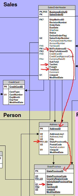
The Adventure Works database has been released alongside every new version of Microsoft SQLServer, and is a large and normalized database (full diagram from blog.jpries) that covers the sales, production, and purchasing of a fictional manufacturer.
For this article, we are going to focus on the SalesOrderHeaders table. Specifically, we want to analyze how much is being purchased in each state, and the average tax rate.

The SalesOrderHeader directly contains the “TaxAmt” and “TotalDue” fields, so that can easily be used in our analysis. But notice there is no state field, instead “BillToAddressId” is normalized into another table.
So we will need to resolve BillToAddressId to a state name. But notice, there is an even deeper level of normalization, because that table uses “StateProvinceID” to look into the “StateProvince” table for the actual state name.
Luckily, the pandas merge method can help us perform these operations.
Download scripts and data
Download the scripts I have provided on github for fetching the CSV files and running the Python3 pandas script.
# make sure wget is installed
sudo apt install wget -y

# download bash script that fetches data
wget https://raw.githubusercontent.com/fabianlee/blogcode/master/pandas/flatten_relational/fetch_relational_data.sh

# download Python3 script that flattens data
https://raw.githubusercontent.com/fabianlee/blogcode/master/pandas/flatten_relational/flatten_relational.py3

# make scripts executable
chmod +x fetch_relational_data.sh
chmod +x flatten_relational.py3
Then fetch the CSV files from the github location.
# fetch the required CSV files for Sales, Address, State tables
./fetch_relational_data.sh
This will retrieve, then do the minimal cleaning necessary to use these files from pandas (converting utf-16 to utf-8).
Install Python3 pandas module
Make sure the pandas module is installed and available to Python3.
pip3 install pandas --user
Run Python3 pandas script
Before I explain the critical pieces of code, let’s run the script and view the final results.
# run script as smoke test
$ ./flatten_relational.py3

Processing 500 max sales rows, debug=False


=== TOTAL TAX AND SALES BY STATE =======================
                  taxamt totaldue meantaxrate
state.name
Arizona            $1.2k   $14.6k       0.085
Bayern             $1.4k   $19.8k       0.072
Brandenburg        $0.3k    $4.0k       0.072
British Columbia  $14.4k  $177.9k       0.081
California        $61.9k  $756.9k       0.082
...                  ...      ...         ...
Virginia           $3.3k   $39.1k       0.085
Washington        $33.2k  $400.9k       0.083
Wisconsin          $1.2k   $13.7k       0.085
Wyoming            $7.2k   $84.8k       0.085
Yveline            $0.9k   $11.9k       0.072

[54 rows x 3 columns]
This shows the total amount of tax and total purchase costs from each state. Along with a synthesized column showing the average tax rate.
This was constructed by reading in the main SalesOrderHeader.csv file, and then resolving address and State foreign keys for a flattened view that can be grouped by State as shown above.
Now let’s go into more detail on how this is done via pandas.
Load DataFrame from CSV file
The ‘read_csv‘ function provides a convenient way of reading a CSV file into a DataFrame.
sales_data = pd.read_csv("SalesOrderHeader.csv",encoding="unicode_escape",sep="\t",nrows=rows)

address_data = pd.read_csv("Address.csv",encoding="unicode_escape",sep="\t")

state_data = pd.read_csv("StateProvince8.csv",encoding="unicode_escape",sep="\t",on_bad_lines="warn",header=0)
We load each of the relational tables into its own DataFrame.
Assign columns to DataFrame
Some CSV files contain header column names, but this particular set does not have them, so we assign names for our convenience.
# define columns since these files do not have headers
# prefixed names (e.g "add." "state.") makes it easier to identify join source later

address_data.columns = ["add.id","add.line1","add.line2","add.city","add.state","add.postalcode","add.spatialloc","add.guid","add.modifieddate"]

state_data.columns = ["state.id","state.code","state.regioncode","state.isstateprovince","state.name","state.territoryid","state.guid","state.modifieddata"]

sales_data.columns = ["id","revision","orderdate","duedate","shipdate","status","onlineflag","salesnum","ponum","acctnum","custid","salespersonid","territoryid","billtoaddressid","shiptoaddressid","shipmethodid","ccid","ccapproval","currencyrateid","subtotal","taxamt","freight","totaldue","comment","guid","modifieddate"]
This knowledge of the format/order usually comes from your DBA group, in our case we have referred to the schema pdf, pdf explanation, and the sql load file.
Flatten Address to include State
The Address table contains a ‘StateProvinceID’ field instead of the State name, so we need to do an inner join to flatten out the DataFrame.
# inner join on Address add.state-> state.stateid
address_data = pd.merge(address_data,state_data,how="left",left_on="add.state",right_on="state.id",suffixes=(None,"_s") )
The address_data DataFrame now contains State name information (col=”state.name”).
Flatten Sales to include Address
The SalesOrderHeader table contains a ‘BillToAddressId’ field instead of the State name, so we need to do an inner join to flatten out the DataFrame.
# inner join on Sales billtoaddressid -> add.id
sales_data = pd.merge(sales_data,address_data,how="left",left_on="billtoaddressid",right_on="add.id",suffixes=(None,"_a") )
The sales_data DataFrame now contains the State name information (col=”state.name”).
Create DataFrame grouping
With all this flattening, our sales_data DataFrame now has a lot of columns. Too many for a compact display of data, so we will create a new DataFrame with just the columns we want to analyze and display.
From this DataFrame, we will group by ‘state.name’, and then create a new synthesized column ‘meantaxrate’ containing the average tax rate for the state.
# select new DataFrame, with just a few columns we want to analyze
sales_data_select_columns = sales_data[ ["state.name", "taxamt", "totaldue"] ]

# sum up the total taxes and purchased, by State
flattened_and_grouped = sales_data_select_columns.groupby(['state.name']).sum()

# create synthesized mean tax rate column based on tax/total
flattened_and_grouped = flattened_and_grouped.assign(meantaxrate = lambda x: x['taxamt']/x['totaldue'] )
If we were just doing data analyis, we would probably stop here and use ‘to_csv‘ to save the results.
Format column data
Since we want to display it on the console, we will format the columns for easier viewing.
First we transform the columns for tax and total amount with a dollar sign and “k” for currency. Then we change the tax rate to show 3 significant digits after the decimal point.
# format tax and total columns into currency for viewing
for col in ['taxamt','totaldue']:
  flattened_and_grouped[col] = flattened_and_grouped[col].apply(lambda x: "${:.1f}k".format((x/1000)))

# format tax rate float to 3 significant decimal points
flattened_and_grouped['meantaxrate'] = flattened_and_grouped['meantaxrate'].apply(lambda x: "{0:.3f}".format(x) )
Display DataFrame
Finally, we show the DataFrame summary of 10 rows.
# show 10 row summary of DataFrame
with pd.option_context('display.max_rows',10):
  print(flattened_and_grouped)
REFERENCES
pandas, merge dataframes explanation
pandas, merge method documentation
pandas, indexing and selecting
github microsoft, Adventure Works CSV files
blog.jpries, Adventure Works explanation
blog.jpries, AdventureWorks schema illustrated as PDF
dataedo.com, pdf explains each field in Adventure Works
svitla.com, dataframes and joining with pandas with diagram of join types
askpython, pandas option_context to show certain row count
stackovervflow, dataframe select versus copy
datagy.io, pandas select and copy
re-thought.com, adding new column in dataframe